IRT Tutorial
Item Response Theory
In this tutorial, I will show how to conduct Item Response Theory models to assess the psychometric structure of typical eyewitness memory assessements (e.g., DRM, misinformation). I will focus on IRT models with binary outcomes as this is most typically used in eyewitness memory research. In this tutorial I will use the data of Otgaar et al. (2020) - False denials. In this tutorial, I will show how to:
- Conduct a Rasch model
- Features to inspect
- Extracting underlying factor scores
Load Data
We will start with 1 DRM list of the study of Otgaar et al (2020). We will focus on true memory (studied items).
# Load data
df <- read_sav("False_Denials_sav_2.sav")

# Create dataframe
df <- as.data.frame(df)

# First DRM list
rel <- df %>% dplyr::select(Table, Sit, Leg, Seat, Couch)
head(rel)
##   Table Sit Leg Seat Couch
## 1    NA  NA  NA   NA    NA
## 2     1   1   0    1     1
## 3     1   1   0    1     1
## 4     1   1   1    1     1
## 5     1   0   1    1     1
## 6     1   1   0    1     1
Classic reliability analysis
splitHalf(rel)
## Split half reliabilities
## Call: splitHalf(r = rel)
##
## Maximum split half reliability (lambda 4) =  0.55
## Guttman lambda 6                          =  0.48
## Average split half reliability            =  0.49
## Guttman lambda 3 (alpha)                  =  0.51
## Guttman lambda 2                          =  0.53
## Minimum split half reliability  (beta)    =  0.37
## Average interitem r =  0.17  with median =  0.21
Rasch Model
We can also analyze this via the IRT. Let’s first conduct a Rasch model. A Rasch model only examines the difficulty (i.e., how good does your memory latent trait have to be to answer the answer correctly) of the items but not how well they discriminate (i.e., how well the item discriminates between people with different latent trait levels of memory). In other words, it only estimate one parameter (1PL). 2PL models also asses the discriminability of the items ()
# Create subset for 1st list
df_irt <- df %>% dplyr::select(Table, Sit, Leg, Seat, Couch)

#  First remove first row of NAs
df_irt <- na.omit(df_irt)

# Conduct Rasch model
mod_rasch <- mirt(df_irt,1, itemtype = "Rasch", verbose=F)

# Results
mod_rasch
##
## Call:
## mirt(data = df_irt, model = 1, itemtype = "Rasch", verbose = F)
##
## Full-information item factor analysis with 1 factor(s).
## Converged within 1e-04 tolerance after 42 EM iterations.
## mirt version: 1.42
## M-step optimizer: nlminb
## EM acceleration: Ramsay
## Number of rectangular quadrature: 61
## Latent density type: Gaussian
##
## Log-likelihood = -360.5729
## Estimated parameters: 6
## AIC = 733.1458
## BIC = 750.7956; SABIC = 731.8124
## G2 (25) = 33.86, p = 0.1109
## RMSEA = 0.051, CFI = NaN, TLI = NaN
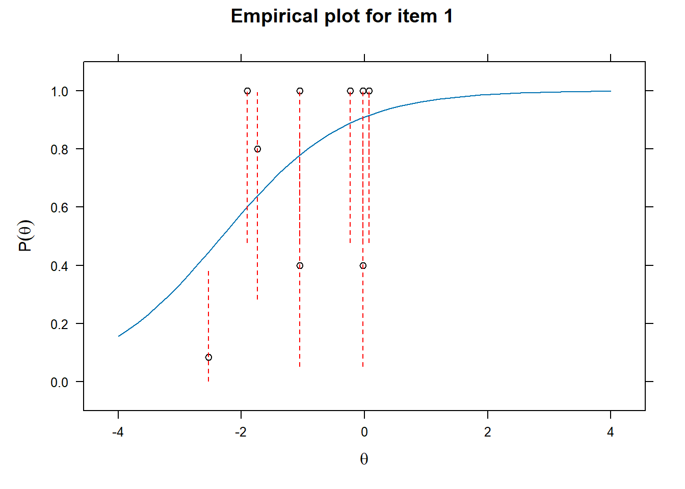
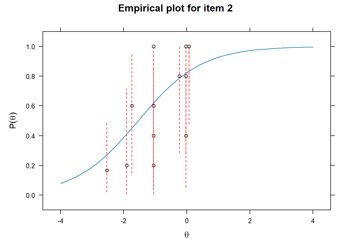
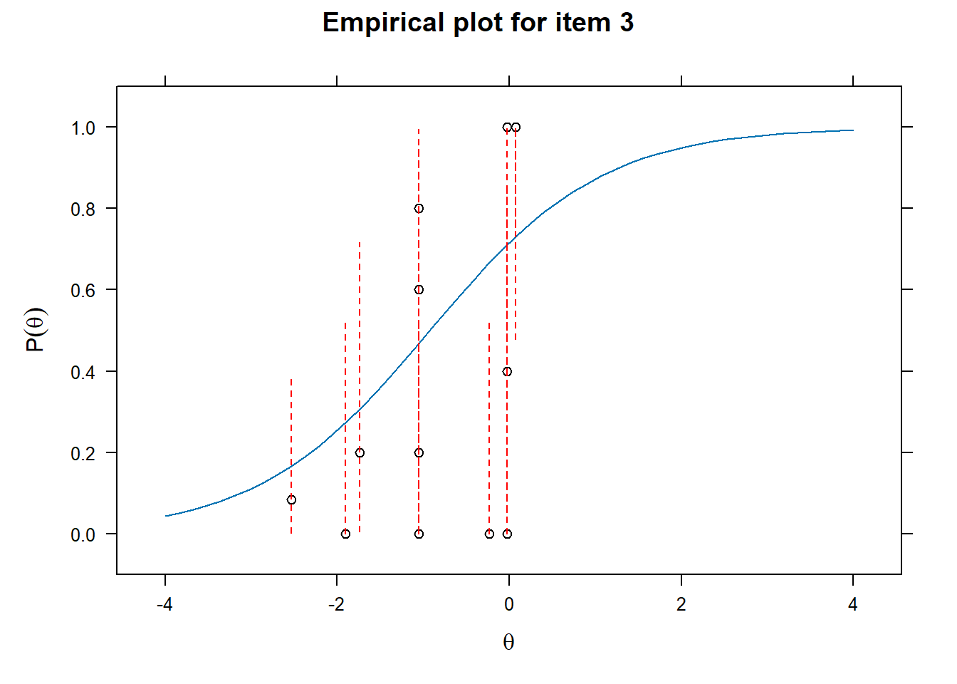
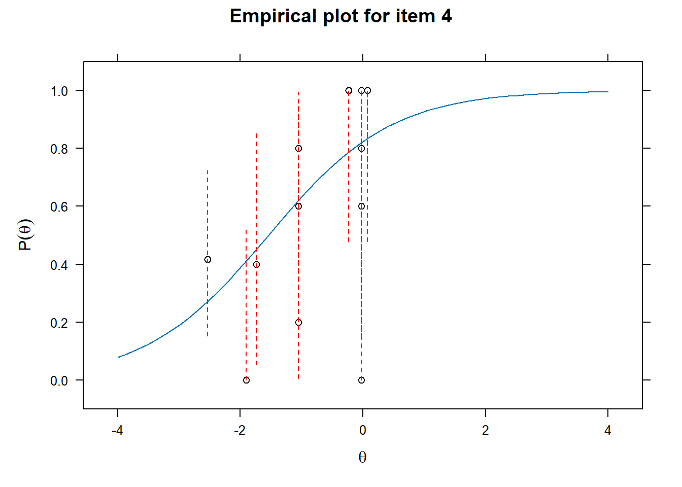
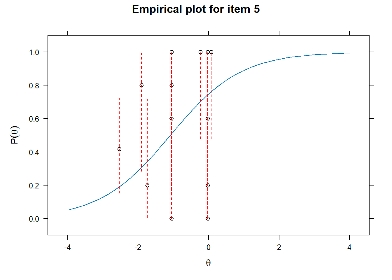
Examining fit of individual items
- This will provide information on how well the datapoints are distributed along the line.
# Examine item fit
for (i in 1:length(df_irt)){
  ItemPlot <- itemfit(mod_rasch,
                      group.bins = 25,
                      empirical.plot = i,
                      empirical.CI = .95,
                      method = "ML")
  print(ItemPlot)
}
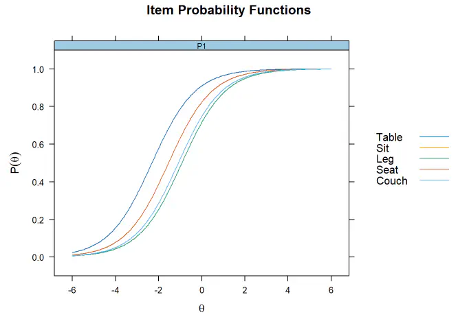
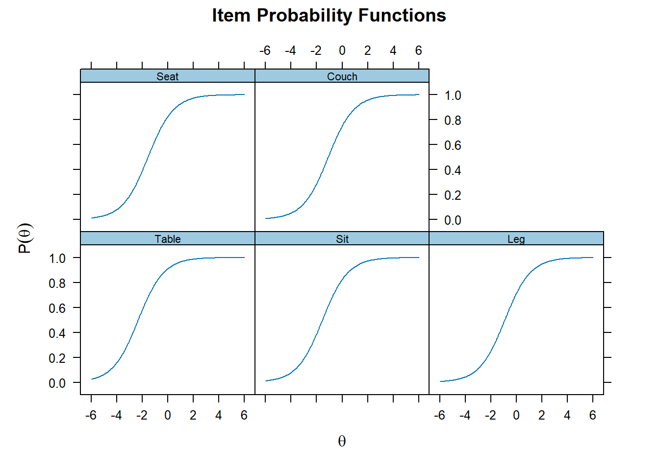
Plot the individual items - Difficulty
- Because we conduct a Rasch model, discriminability is constrained to 1. This can be seen by the identitical curves for each items
# Item specific graphs
plot(mod_rasch, type = "trace")
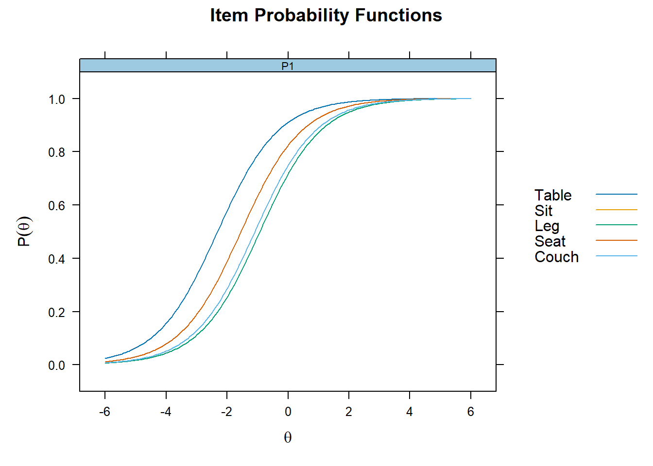
Plot together
plot(mod_rasch,type= "trace", facet_items=F)
Coefficients
- Difficulty can be seen as how much latent trait ability is necessary to endorse the item.
- In terms of coefficients, it is the latent trait ability level at which there is .50 probability of endorsing the item (indicating yes/remember, etc)
# Get item coefficients
# To get the easy parameter change "IRTpars = F"
coef(mod_rasch, IRTpars = T, simplify = T)
## $items
##       a      b g u
## Table 1 -2.312 0 1
## Sit   1 -1.542 0 1
## Leg   1 -0.923 0 1
## Seat  1 -1.542 0 1
## Couch 1 -1.087 0 1
##
## $means
## F1
##  0
##
## $cov
##       F1
## F1 1.208
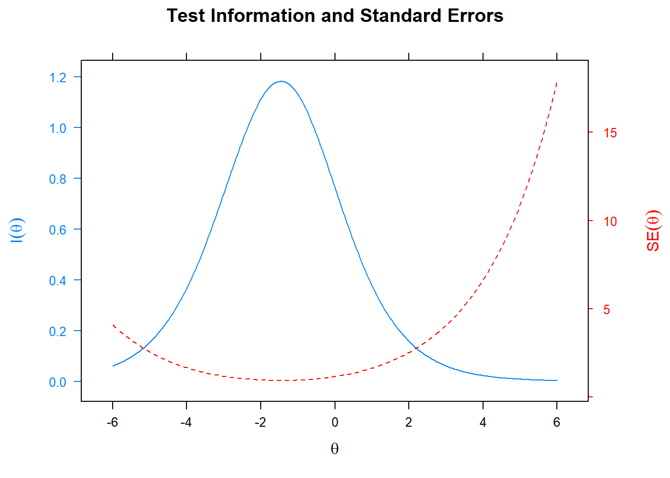
Information of the test
- Specifically, this provide a plot at which levels of the latent trait ability the test is most informative
- Plotting the standard error also indicates where the standard error is largest for the specific test.
plot(mod_rasch, type= "infoSE")
Factor scores
# Get latent trait scores
df_irt$fscor <- mirt::fscores(mod_rasch)
head(df_irt$fscor)
##              F1
## [1,] 0.06590852
## [2,] 0.06590852
## [3,] 0.77109655
## [4,] 0.06590852
## [5,] 0.06590852
## [6,] 0.77109655