ROC Curve Brady et al. (2022)

Paul Riesthuis

Last updated on Sep 23, 2023 7 min read ROC

ROC cuve analysis of Brady et al. (2022).

In this blogpost, I will show how to construct the datasets of Tim and John and the Receiver Operator Characteristic (ROC) curves provided in the article of Brady et al. (2022)
- Then, I will show the following:
  - How to calculate common statistics that can be calculated based on this type of dataset. Most statistics are similar to the ones shown at the page about “old” and “new” memory task
  - How to construct (ROC) curves by hand and via logistic regression.
  - How to calculate the area under the ROC curve.
  - How to calculate confidence intervals for the AUC
  - How to calculate partial area under the curve.

Datasets constructed by hand

Dataset of Tim

old_items_tim <- c(50,50,50,150,500,200)
new_items_tim <- c(250,250,400,50,25,25)
confidence <- c("extreme weak","very weak", "fairly weak", "fairly strong", "very strong", "extreme strong")
df_tim <- data.frame(old_items_tim, new_items_tim, confidence)
nice_table(df_tim,
           title= "Dataset for Tim")

Dataset for Tim
old_items_tim	new_items_tim	confidence
50.00	250.00	extreme weak
50.00	250.00	very weak
50.00	400.00	fairly weak
150.00	50.00	fairly strong
500.00	25.00	very strong
200.00	25.00	extreme strong

Dataset John

old_items_john <- c(50,75,75,500,200,100)
new_items_john <- c(100,400,300,50,75,75) # changed very strong to 75 instead of 25 to have equal number items between tim and john
df_john <- data.frame(old_items_john, new_items_john, confidence)
nice_table(df_john,
           title = "Dataset for John")

Dataset for John
old_items_john	new_items_john	confidence
50.00	100.00	extreme weak
75.00	400.00	very weak
75.00	300.00	fairly weak
500.00	50.00	fairly strong
200.00	75.00	very strong
100.00	75.00	extreme strong

Add hit rate and false alarm rate

Tim

#hit rates Tim
tot_items_tim <- sum(old_items_tim) # to get the total amount of items
df_tim$hit <- c(old_items_tim[1]/tot_items_tim, 
         (old_items_tim[1]+old_items_tim[2])/tot_items_tim,
         (old_items_tim[1]+old_items_tim[2]+old_items_tim[3])/tot_items_tim,
         (old_items_tim[1]+old_items_tim[2]+old_items_tim[3]+old_items_tim[4])/tot_items_tim,
         (old_items_tim[1]+old_items_tim[2]+old_items_tim[3]+old_items_tim[4]+old_items_tim[5])/tot_items_tim,
         (old_items_tim[1]+old_items_tim[2]+old_items_tim[3]+old_items_tim[4]+old_items_tim[5]+old_items_tim[6])/tot_items_tim)
        
  
#false alarm rate Tim
tot_new_tim <- sum(new_items_tim)
df_tim$far <- c(new_items_tim[1]/tot_new_tim, 
         (new_items_tim[1]+new_items_tim[2])/tot_new_tim,
         (new_items_tim[1]+new_items_tim[2]+new_items_tim[3])/tot_new_tim,
         (new_items_tim[1]+new_items_tim[2]+new_items_tim[3]+new_items_tim[4])/tot_new_tim,
         (new_items_tim[1]+new_items_tim[2]+new_items_tim[3]+new_items_tim[4]+new_items_tim[5])/tot_new_tim,
         (new_items_tim[1]+new_items_tim[2]+new_items_tim[3]+new_items_tim[4]+new_items_tim[5]+new_items_tim[6])/tot_new_tim)
nice_table(df_tim,
           title= "Dataset + Hit and False Alarm rate for Tim")

Dataset + Hit and False Alarm rate for Tim
old_items_tim	new_items_tim	confidence	hit	far
50.00	250.00	extreme weak	0.05	0.25
50.00	250.00	very weak	0.10	0.50
50.00	400.00	fairly weak	0.15	0.90
150.00	50.00	fairly strong	0.30	0.95
500.00	25.00	very strong	0.80	0.97
200.00	25.00	extreme strong	1.00	1.00

John

#hit rates for john
tot_old_john <- sum(old_items_john)
df_john$hit <- c(old_items_john[1]/tot_old_john, 
         (old_items_john[1]+old_items_john[2])/tot_old_john,
         (old_items_john[1]+old_items_john[2]+old_items_john[3])/tot_old_john,
         (old_items_john[1]+old_items_john[2]+old_items_john[3]+old_items_john[4])/tot_old_john,
         (old_items_john[1]+old_items_john[2]+old_items_john[3]+old_items_john[4]+old_items_john[5])/tot_old_john,
         (old_items_john[1]+old_items_john[2]+old_items_john[3]+old_items_john[4]+old_items_john[5]+old_items_john[6])/tot_old_john)

# false alarm rate john
tot_new_john <- sum(new_items_john)
df_john$far <- c(new_items_john[1]/tot_new_john, 
         (new_items_john[1]+new_items_john[2])/tot_new_john,
         (new_items_john[1]+new_items_john[2]+new_items_john[3])/tot_new_john,
         (new_items_john[1]+new_items_john[2]+new_items_john[3]+new_items_john[4])/tot_new_john,
         (new_items_john[1]+new_items_john[2]+new_items_john[3]+new_items_john[4]+new_items_john[5])/tot_new_john,
         (new_items_john[1]+new_items_john[2]+new_items_john[3]+new_items_john[4]+new_items_john[5]+new_items_john[6])/tot_new_john)
nice_table(df_john,
           title= "Dataset + Hit and False Alarm rate for John")

Dataset + Hit and False Alarm rate for John
old_items_john	new_items_john	confidence	hit	far
50.00	100.00	extreme weak	0.05	0.10
75.00	400.00	very weak	0.12	0.50
75.00	300.00	fairly weak	0.20	0.80
500.00	50.00	fairly strong	0.70	0.85
200.00	75.00	very strong	0.90	0.92
100.00	75.00	extreme strong	1.00	1.00

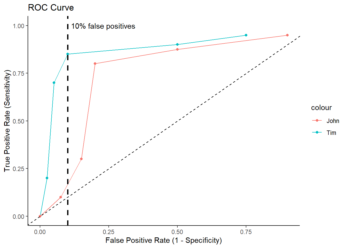
Plot ROC Curves for Tim and John

roc_data <- data.frame(df_tim,df_john)
ggplot(roc_data, aes(x = 1- far, y = 1- hit, color = "Tim")) +
  geom_line()+ geom_point()+
  geom_line(aes(x = 1 - far.1, y = 1 - hit.1, color="John"))+ geom_point(aes(x = 1 - far.1, y = 1 - hit.1, color="John"))+
  geom_abline(intercept = 0, slope = 1, linetype = "dashed") +
  labs(x = "False Positive Rate (1 - Specificity)", y = "True Positive Rate (Sensitivity)") +
  ggtitle("ROC Curve")+
  theme_classic()+
  ylim(0,1)+
  geom_vline(xintercept = .10,
             lwd = 1,
             linetype="dashed")+
  annotate("text", x=.23, y=1, label="10% false positives")

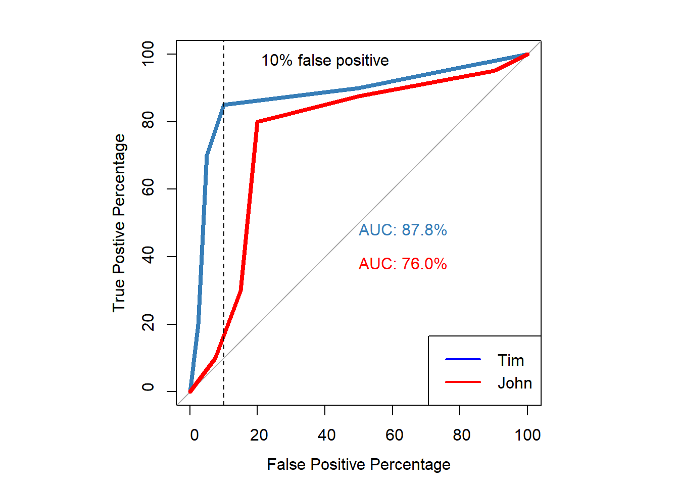
ROC Curve via Logistic regression

Create datasets for Tim and John that are compatible for logistic regression.

correct_mem <- rep(c(1, 0), each = 1000)
confidence_tim  <- c(rep(1,50),
                 rep(2,50),
                 rep(3,50),
                 rep(4,150),
                 rep(5,500),
                 rep(6,200),
                 rep(1,250),
                 rep(2,250),
                 rep(3,400),
                 rep(4,50),
                 rep(5,25),
                 rep(6,25))
confidence_john  <- c(rep(1,50),
                 rep(2,75),
                 rep(3,75),
                 rep(4,500),
                 rep(5,200),
                 rep(6,100),
                 rep(1,100),
                 rep(2,400),
                 rep(3,300),
                 rep(4,50),
                 rep(5,75), # i made this 75 as in the article there are otherwise only 1950 items for john instead 2000 as with Tim's. It was orignally 25
                 rep(6,75))
df <- data.frame(correct_mem,confidence_tim,confidence_john)

Create ROC Curves for both

glm.fit_tim=glm(correct_mem ~ confidence_tim, family=binomial)
glm.fit_john=glm(correct_mem ~ confidence_john, family=binomial)

par(pty="s")
p1 <- roc(correct_mem, glm.fit_tim$fitted.values, 
    plot= TRUE,
    legacy.axes=TRUE, 
    percent=TRUE, 
    xlab="False Positive Percentage", 
    ylab="True Postive Percentage", 
    col="#377eb8", 
    lwd=4,
    print.auc = TRUE)

p2 <- roc(correct_mem, glm.fit_john$fitted.values, 
    plot= TRUE,
    legacy.axes=TRUE, 
    percent=TRUE, 
    xlab="False Positive Percentage", 
    ylab="True Postive Percentage", 
    col="red", 
    lwd=4,
    print.auc = TRUE,
    print.auc.y = 40,
    add=TRUE)
abline(v = 90, col = "black", lty = 2)
text(x = 60, y = 98, labels = "10% false positive", col = "black")
legend("bottomright", legend=c("Tim", "John"),
       col=c("Blue","red"), lwd=2)

True and False Positive per Threshold

This can be used to examine the blackstone ratio (10:1; false negative to false positive ratio)
True and False Positive percentages for each confidence threshold for Tim

info_tim <- roc(correct_mem, glm.fit_tim$fitted.values) 
tim.df <- data.frame(
  Confidence = c("","Extreme-very weak", "Very-fairly weak", "Weak-strong", "Fairly-very strong","Very-extreme strong",""),
  tpp=info_tim$sensitivities*100,
  fpp=(1-info_tim$specificities)*100, #to make sure the order goes from weak to high confidence
  thresholds = info_tim$thresholds,
  FN_FP = (length(info_tim$cases)*(1-info_tim$sensitivities))/(length(info_tim$controls)*(1-info_tim$specificities)))

tim.df <- tim.df[-c(1,7), ]  
nice_table(tim.df,
           title="True Positive and False Positive Percentages for each Threshold")

True Positive and False Positive Percentages for each Threshold
Confidence	tpp	fpp	thresholds	FN_FP
Extreme-very weak	95.00	75.00	0.09	0.07
Very-fairly weak	90.00	50.00	0.24	0.20
Weak-strong	85.00	10.00	0.49	1.50
Fairly-very strong	70.00	5.00	0.75	6.00
Very-extreme strong	20.00	2.50	0.90	32.00

True and False Positive percentages for each confidence threshold for John

info_john <- roc(correct_mem, glm.fit_john$fitted.values) 
john.df <- data.frame(
  Confidence = c("","Extreme-very weak", "Very-fairly weak", "Weak-strong", "Fairly-very strong","Very-extreme strong",""),
  tpp=info_john$sensitivities*100,
  fpp=(1-info_john$specificities)*100, #to make sure the order goes from weak to high confidence
  thresholds = info_john$thresholds,
  FN_FP = (length(info_john$cases)*(1-info_john$sensitivities))/(length(info_john$controls)*(1-info_john$specificities)))

john.df <- john.df[-c(1,7), ]  
nice_table(john.df,
           title="True Positive and False Positive Percentages for each Threshold for John")

True Positive and False Positive Percentages for each Threshold for John
Confidence	tpp	fpp	thresholds	FN_FP
Extreme-very weak	95.00	90.00	0.21	0.06
Very-fairly weak	87.50	50.00	0.35	0.25
Weak-strong	80.00	20.00	0.51	1.00
Fairly-very strong	30.00	15.00	0.68	4.67
Very-extreme strong	10.00	7.50	0.81	12.00

Confidence Intervals

The graphs provide important information for whos memory is better.
- For example, the ROC curve of Tim is greater at eacg threshold than the ROC curve of John.
However, to fully examine the AUC we would like 95% CI.
- This can be easily extracted in the pROC package.
- You can either choose to bootstrap or use the delong method.
- Using the 95%CI the AUC can be compared to the smallest effect size of interest (e.g., AUC_null = .8).

# Delong method
auc_tim <- roc(correct_mem, glm.fit_tim$fitted.values)
auc_john <- roc(correct_mem, glm.fit_john$fitted.values)
CI_delong_tim <- ci.auc(auc_tim) # default is 95%
CI_delong_john <- ci.auc(auc_john) 
CI_boot_tim <- ci.auc(auc_tim, method = "bootstrap", boot.n = 1000) # bootstrapping 1000 times
CI_boot_john <- ci.auc(auc_john, method = "bootstrap", boot.n = 1000) # bootstrapping 1000 times
p_tim <- power.roc.test(auc_tim) # null hypothesis is set to .5
p_john <- power.roc.test(auc_john)# null hypothesis is set to .5
tab_ci <- data.frame(
  Name = c("Tim","John"),
  AUC = c(CI_delong_tim[2],CI_delong_john[2]), #AUC values
  CI_low_Delong = c(CI_delong_tim[1],CI_delong_john[1]), # lower bound CI delong
  CI_upper_Delong = c(CI_delong_tim[3],CI_delong_john[3]),# upper bound CI delong
  CI_low_boot = c(CI_delong_tim[1],CI_delong_john[1]),# lower bound CI bootstrap
  CI_upper_boot = c(CI_delong_tim[3],CI_delong_john[3]),# upper bound CI bootstrap
  Power = c(p_tim$power,p_john$power)
)
nice_table(tab_ci,
           title = "AUC values with 95% CI via Delong or bootstrapping",
)

AUC values with 95% CI via Delong or bootstrapping
Name	AUC	CI_low_Delong	CI_upper_Delong	CI_low_boot	CI_upper_boot	Power
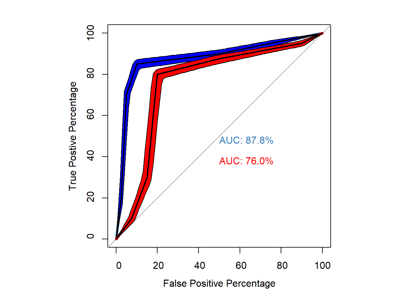
Tim	0.88	0.86	0.89	0.86	0.89	1.00
John	0.76	0.74	0.78	0.74	0.78	1.00

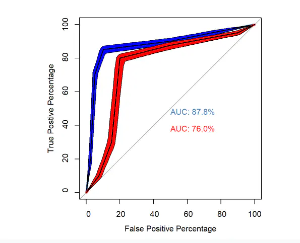
ROC curves with 95%

Preferably, we plot the confidence intervals along the ROC curve to better interpret the results

par(pty="s")
p1 <- roc(correct_mem, glm.fit_tim$fitted.values, 
    plot= TRUE,
    legacy.axes=TRUE, 
    percent=TRUE, 
    xlab="False Positive Percentage", 
    ylab="True Postive Percentage", 
    col="#377eb8", 
    lwd=4,
    print.auc = TRUE)
p3 <- ci.se(p1,                         # CI of Tim
            specificities = seq(0, 100, 1),  # CI of sensitivity at at what specificities? 0,5,10,15,....,100
            conf.level=0.95,                 # level of Confidence interval
) 

plot(p3, type = "shape", col = "blue")

p2 <- roc(correct_mem, glm.fit_john$fitted.values, 
    plot= TRUE,
    legacy.axes=TRUE, 
    percent=TRUE, 
    xlab="False Positive Percentage", 
    ylab="True Postive Percentage", 
    col="red", 
    lwd=4,
    print.auc = TRUE,
    print.auc.y = 40,
    add=TRUE)
p4 <- ci.se(p2,                         # CI of john 
            specificities = seq(0, 100, 1),  # CI at which thresholds?
            conf.level=0.95,                 # indicate confidence interval
) 
plot(p4, type = "shape", col = "red")     # plot as a blue shape

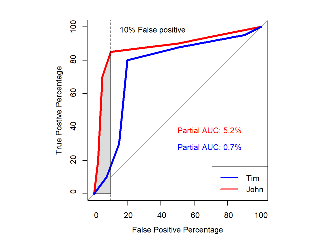
Partial AUC

We can calculate the area under the curve for a part of the curve.
- One example is to calculate the curve for values under the 10% false positive
- That is because we want to minimize the amount of false positive when it comes to eyewitness identification.

# Calculate the partial AUC
partial_auc_tim <- roc(correct_mem, glm.fit_tim$fitted.values, partial.auc=c(100,90), percent = T)
partial_auc_john <- roc(correct_mem, glm.fit_john$fitted.values, partial.auc=c(100,90), percent = T)

# Print the partial AUC
par(pty="s")
p1 <- plot(partial_auc_tim,
    plot= TRUE,
    legacy.axes=TRUE, 
    xlab="False Positive Percentage", 
    ylab="True Postive Percentage", 
    col="red", 
    lwd=4,
    print.auc = TRUE,
    print.auc.x = 50,
    print.auc.y = 40,
    auc.polygon=TRUE,
    percent=TRUE)
p1 <- plot(partial_auc_john,
    plot= TRUE,
    legacy.axes=TRUE, 
    xlab="False Positive Percentage", 
    ylab="True Postive Percentage", 
    col="blue", 
    lwd=4,
    print.auc = TRUE,
    print.auc.x = 50,
    print.auc.y = 30,
    auc.polygon=TRUE,
    percent=TRUE,
    add=T)
abline(v = 90, col = "black", lty = 2)
text(x = 65, y = 98, labels = "10% False positive", col = "black")
legend("bottomright", legend=c("Tim", "John"),
       col=c("Blue","red"), lwd=2)