Safe Testing
Safe Testing
Safe testing is a statistical analysis that allows researchers to analyze the data at any moment without have to worry about alpha corrections. This means that the researchers can look at their data at any time to see if they found meaningful differences. In this blogpost, I will show how:
- safe testing can be conducted in R.
- I will show that it indeed does not lead to an inflated type 1 error rate which is observed in traditional hypothesis significance testing.
- I will show how the any time valid confidence sequences can be used.
- I will propose a way in how the any time valid confidence sequences can be used as a form of equivalence and minimum-effect testing.
Safe Testing - Independent sample t-test
To conduct a safe test for an independent sample t-test we need the following information:
- Alpha
- Beta
- Smallest effect size of interest = SESOI
Using these parameters, we can create a designSafeT which is necessary to obtain the e-values and anytime valid confidence sequences
Preparation
##
|
| | 0%
|
| | 1%
|
|= | 1%
|
|= | 2%
|
|== | 2%
|
|== | 3%
|
|== | 4%
|
|=== | 4%
|
|=== | 5%
|
|==== | 5%
|
|==== | 6%
|
|===== | 6%
|
|===== | 7%
|
|===== | 8%
|
|====== | 8%
|
|====== | 9%
|
|======= | 9%
|
|======= | 10%
|
|======= | 11%
|
|======== | 11%
|
|======== | 12%
|
|========= | 12%
|
|========= | 13%
|
|========= | 14%
|
|========== | 14%
|
|========== | 15%
|
|=========== | 15%
|
|=========== | 16%
|
|============ | 16%
|
|============ | 17%
|
|============ | 18%
|
|============= | 18%
|
|============= | 19%
|
|============== | 19%
|
|============== | 20%
|
|============== | 21%
|
|=============== | 21%
|
|=============== | 22%
|
|================ | 22%
|
|================ | 23%
|
|================ | 24%
|
|================= | 24%
|
|================= | 25%
|
|================== | 25%
|
|================== | 26%
|
|=================== | 26%
|
|=================== | 27%
|
|=================== | 28%
|
|==================== | 28%
|
|==================== | 29%
|
|===================== | 29%
|
|===================== | 30%
|
|===================== | 31%
|
|====================== | 31%
|
|====================== | 32%
|
|======================= | 32%
|
|======================= | 33%
|
|======================= | 34%
|
|======================== | 34%
|
|======================== | 35%
|
|========================= | 35%
|
|========================= | 36%
|
|========================== | 36%
|
|========================== | 37%
|
|========================== | 38%
|
|=========================== | 38%
|
|=========================== | 39%
|
|============================ | 39%
|
|============================ | 40%
|
|============================ | 41%
|
|============================= | 41%
|
|============================= | 42%
|
|============================== | 42%
|
|============================== | 43%
|
|============================== | 44%
|
|=============================== | 44%
|
|=============================== | 45%
|
|================================ | 45%
|
|================================ | 46%
|
|================================= | 46%
|
|================================= | 47%
|
|================================= | 48%
|
|================================== | 48%
|
|================================== | 49%
|
|=================================== | 49%
|
|=================================== | 50%
|
|=================================== | 51%
|
|==================================== | 51%
|
|==================================== | 52%
|
|===================================== | 52%
|
|===================================== | 53%
|
|===================================== | 54%
|
|====================================== | 54%
|
|====================================== | 55%
|
|======================================= | 55%
|
|======================================= | 56%
|
|======================================== | 56%
|
|======================================== | 57%
|
|======================================== | 58%
|
|========================================= | 58%
|
|========================================= | 59%
|
|========================================== | 59%
|
|========================================== | 60%
|
|========================================== | 61%
|
|=========================================== | 61%
|
|=========================================== | 62%
|
|============================================ | 62%
|
|============================================ | 63%
|
|============================================ | 64%
|
|============================================= | 64%
|
|============================================= | 65%
|
|============================================== | 65%
|
|============================================== | 66%
|
|=============================================== | 66%
|
|=============================================== | 67%
|
|=============================================== | 68%
|
|================================================ | 68%
|
|================================================ | 69%
|
|================================================= | 69%
|
|================================================= | 70%
|
|================================================= | 71%
|
|================================================== | 71%
|
|================================================== | 72%
|
|=================================================== | 72%
|
|=================================================== | 73%
|
|=================================================== | 74%
|
|==================================================== | 74%
|
|==================================================== | 75%
|
|===================================================== | 75%
|
|===================================================== | 76%
|
|====================================================== | 76%
|
|====================================================== | 77%
|
|====================================================== | 78%
|
|======================================================= | 78%
|
|======================================================= | 79%
|
|======================================================== | 79%
|
|======================================================== | 80%
|
|======================================================== | 81%
|
|========================================================= | 81%
|
|========================================================= | 82%
|
|========================================================== | 82%
|
|========================================================== | 83%
|
|========================================================== | 84%
|
|=========================================================== | 84%
|
|=========================================================== | 85%
|
|============================================================ | 85%
|
|============================================================ | 86%
|
|============================================================= | 86%
|
|============================================================= | 87%
|
|============================================================= | 88%
|
|============================================================== | 88%
|
|============================================================== | 89%
|
|=============================================================== | 89%
|
|=============================================================== | 90%
|
|=============================================================== | 91%
|
|================================================================ | 91%
|
|================================================================ | 92%
|
|================================================================= | 92%
|
|================================================================= | 93%
|
|================================================================= | 94%
|
|================================================================== | 94%
|
|================================================================== | 95%
|
|=================================================================== | 95%
|
|=================================================================== | 96%
|
|==================================================================== | 96%
|
|==================================================================== | 97%
|
|==================================================================== | 98%
|
|===================================================================== | 98%
|
|===================================================================== | 99%
|
|======================================================================| 99%
|
|======================================================================| 100%
Then we have sufficient information to run the safe t test.
Create datasets
Let’s create a dataset for a two group experimental between subjects design.
# Generate a dataset for each group
group1 <- rnorm(150,7,2)
group2 <- rnorm(150,6,2)

# Show first 5 rows
head(group1)
## [1] 6.615987 6.820546 10.967876 7.231223 4.882142 6.557919
head(group2)
## [1] 8.419868 7.177548 6.530180 5.572583 6.766534 7.805942
Normal independent sample t-test
t.test(x=group1,
       y=group2,
       alternative = "two.sided",
       paired=FALSE)
##
## 	Welch Two Sample t-test
##
## data:  group1 and group2
## t = 2.2176, df = 292.65, p-value = 0.02735
## alternative hypothesis: true difference in means is not equal to 0
## 95 percent confidence interval:
##  0.0592708 0.9944163
## sample estimates:
## mean of x mean of y
##  6.761232  6.234388
This leads to a p-value < .001 and a raw mean difference of 1.1 95%CI[.66, 1.58]
Safe independent sample t-test
safeTTest(x=group1,
          y=group2,
          alternative = "greater",
          designObj=designObj,
          paired=FALSE)
##
## 	Safe Two Sample T-Test
##
## data:  group1 and group2. n1 = 150, n2 = 150
## estimates: mean of x = 6.7612, mean of y = 6.2344
## 95 percent confidence sequence:
##  -0.208491  1.262178
##
## test: t = 2.2176, deltaS = 0.5
## e-value = 1.2631 > 1/alpha = 20 : FALSE
## alternative hypothesis: true difference in means ('x' minus 'y') is greater than 0
##
## design: the test was designed with alpha = 0.05
## for experiments with n1Plan = 75, n2Plan = 75
## to guarantee a power = 0.8 (beta = 0.2)
## for minimal relevant standardised mean difference = 0.5 (greater)
There are no p-values for safe tests but e-values. For e-values, a value above 20 (1/.05) is deemed as evidence for the alternative hypothesis. In this case the e-value is 55038 with a raw mean difference of 1.1 and a 95% any time valid confidence sequence [.40, 1.85].
Hence, the results are the same.
Examine p-values and e-values sequentially
Same steps as above but we now conduct the analysis after each participants data comes in.
# create empty columns for extracted data
evs <- c() # evalues
ps <- c() # pvalues
L95 <- c() # 95 any time valid confidence sequence
H95 <- c() # 95 any time valid confidence sequence
L95CI <- c() # 95 confidence interval
H95CI <- c() # 95 confidence interval
est <- c() # Estimate mean difference

# For loop to conduct analysis after each participant.
for (i in 2:length(group1)) {
  set.seed(2)
  g1 <- head(group1, i)
  g2 <- head(group2, i)
  s <- safeTTest(x=g1, y=g2, alternative = "greater",
            designObj=designObj, paired=FALSE)
  evs[i] <- s$eValue
  e <- t.test(x=g1, y=g2, alternative = "two.sided",
              designObj=designObj, paired=FALSE)
  ps[i] <- e$p.value
  L95[i] <- s$confSeq[1]
  H95[i] <- s$confSeq[2]
  est[i] <- s$estimate[1] - s$estimate[2]
  L95CI[i] <- e$conf.int[1]
  H95CI[i] <- e$conf.int[2]
}

# Put data together
df_error <- data.frame(evs, ps,L95,H95,L95CI,H95CI,est)

# Add a participants variable
df_error$par <- seq(1,length(g1),1)

# Remove first row of data because they are NAs (no comparisons can be done with only 1 participant)
df_error <- na.omit(df_error)

# For safe testing there are no anytime valid confidence sequences for the first 5 comparisons/participants per group.
df_error$L95[!is.finite(df_error$L95)] <- NA # first five comparisons there are no CIs
df_error$H95[!is.finite(df_error$H95)] <- NA # first five comparisons there are no CIs

# Show first 5 rows
head(df_error)
##         evs        ps       L95      H95     L95CI    H95CI        est par
## 2 0.4924300 0.3262269        NA       NA -8.170243 6.009360 -1.0804414   2
## 3 1.1421242 0.6572057        NA       NA -4.539091 6.056967  0.7589376   3
## 4 1.4055865 0.4468779        NA       NA -2.106416 4.074142  0.9838632   4
## 5 0.9910386 0.7233756        NA       NA -2.328884 3.149309  0.4102122   5
## 6 0.7821122 0.8884207        NA       NA -2.026358 2.294037  0.1338396   6
## 7 0.9201306 0.7181550 -7.152289 7.811039 -1.630509 2.289259  0.3293752   7
Plot p-values
ggplot(df_error, aes(x = par, y = ps))+
  geom_point()+
  geom_line(color="red")+
  geom_hline(yintercept= .05, linetype= "dashed", color = "blue", size= 1)+
  theme_barbie()+
  labs(y = "p-values",
       x = "Participants")+
  transition_reveal(seq_along(par)) + shadow_mark()
Plot e-values
ggplot(df_error, aes(x = par, y = evs))+
  geom_point()+
  geom_line()+
  geom_hline(yintercept= 20, linetype= "dashed", color = "red", size= 1)+
  labs(y = "p-values",
       x = "Participants")+
  transition_reveal(seq_along(par)) + shadow_mark()+
  theme_barbie()
Plot raw mean difference and 95%CI and CS
- The lines on the outside reflect the lower and upper any time valid confidence sequences
- The next two lines reflect the lower and upper 95%CIs
- The middle line is the estimate for the raw mean difference
ggplot(df_error, aes(x = par))+
  geom_point(aes(y = L95))+
  geom_line(aes(y = L95))+
  geom_point(aes(y= H95))+
  geom_line(aes(y = H95))+
  geom_point(aes(y = L95CI))+
  geom_line(aes(y = L95CI))+
  geom_point(aes(y= H95CI))+
  geom_line(aes(y = H95CI))+
  geom_point(aes(y = est))+
  geom_line(aes(y = est))+
  transition_reveal(seq_along(par)) + shadow_mark()+
  labs(y = "Raw mean differences",
       x = "Participants")+
  theme_barbie()
Type 1 error inflation check
##
|
| | 0%
|
| | 1%
|
|= | 1%
|
|= | 2%
|
|== | 2%
|
|== | 3%
|
|== | 4%
|
|=== | 4%
|
|=== | 5%
|
|==== | 5%
|
|==== | 6%
|
|===== | 6%
|
|===== | 7%
|
|===== | 8%
|
|====== | 8%
|
|====== | 9%
|
|======= | 9%
|
|======= | 10%
|
|======= | 11%
|
|======== | 11%
|
|======== | 12%
|
|========= | 12%
|
|========= | 13%
|
|========= | 14%
|
|========== | 14%
|
|========== | 15%
|
|=========== | 15%
|
|=========== | 16%
|
|============ | 16%
|
|============ | 17%
|
|============ | 18%
|
|============= | 18%
|
|============= | 19%
|
|============== | 19%
|
|============== | 20%
|
|============== | 21%
|
|=============== | 21%
|
|=============== | 22%
|
|================ | 22%
|
|================ | 23%
|
|================ | 24%
|
|================= | 24%
|
|================= | 25%
|
|================== | 25%
|
|================== | 26%
|
|=================== | 26%
|
|=================== | 27%
|
|=================== | 28%
|
|==================== | 28%
|
|==================== | 29%
|
|===================== | 29%
|
|===================== | 30%
|
|===================== | 31%
|
|====================== | 31%
|
|====================== | 32%
|
|======================= | 32%
|
|======================= | 33%
|
|======================= | 34%
|
|======================== | 34%
|
|======================== | 35%
|
|========================= | 35%
|
|========================= | 36%
|
|========================== | 36%
|
|========================== | 37%
|
|========================== | 38%
|
|=========================== | 38%
|
|=========================== | 39%
|
|============================ | 39%
|
|============================ | 40%
|
|============================ | 41%
|
|============================= | 41%
|
|============================= | 42%
|
|============================== | 42%
|
|============================== | 43%
|
|============================== | 44%
|
|=============================== | 44%
|
|=============================== | 45%
|
|================================ | 45%
|
|================================ | 46%
|
|================================= | 46%
|
|================================= | 47%
|
|================================= | 48%
|
|================================== | 48%
|
|================================== | 49%
|
|=================================== | 49%
|
|=================================== | 50%
|
|=================================== | 51%
|
|==================================== | 51%
|
|==================================== | 52%
|
|===================================== | 52%
|
|===================================== | 53%
|
|===================================== | 54%
|
|====================================== | 54%
|
|====================================== | 55%
|
|======================================= | 55%
|
|======================================= | 56%
|
|======================================== | 56%
|
|======================================== | 57%
|
|======================================== | 58%
|
|========================================= | 58%
|
|========================================= | 59%
|
|========================================== | 59%
|
|========================================== | 60%
|
|========================================== | 61%
|
|=========================================== | 61%
|
|=========================================== | 62%
|
|============================================ | 62%
|
|============================================ | 63%
|
|============================================ | 64%
|
|============================================= | 64%
|
|============================================= | 65%
|
|============================================== | 65%
|
|============================================== | 66%
|
|=============================================== | 66%
|
|=============================================== | 67%
|
|=============================================== | 68%
|
|================================================ | 68%
|
|================================================ | 69%
|
|================================================= | 69%
|
|================================================= | 70%
|
|================================================= | 71%
|
|================================================== | 71%
|
|================================================== | 72%
|
|=================================================== | 72%
|
|=================================================== | 73%
|
|=================================================== | 74%
|
|==================================================== | 74%
|
|==================================================== | 75%
|
|===================================================== | 75%
|
|===================================================== | 76%
|
|====================================================== | 76%
|
|====================================================== | 77%
|
|====================================================== | 78%
|
|======================================================= | 78%
|
|======================================================= | 79%
|
|======================================================== | 79%
|
|======================================================== | 80%
|
|======================================================== | 81%
|
|========================================================= | 81%
|
|========================================================= | 82%
|
|========================================================== | 82%
|
|========================================================== | 83%
|
|========================================================== | 84%
|
|=========================================================== | 84%
|
|=========================================================== | 85%
|
|============================================================ | 85%
|
|============================================================ | 86%
|
|============================================================= | 86%
|
|============================================================= | 87%
|
|============================================================= | 88%
|
|============================================================== | 88%
|
|============================================================== | 89%
|
|=============================================================== | 89%
|
|=============================================================== | 90%
|
|=============================================================== | 91%
|
|================================================================ | 91%
|
|================================================================ | 92%
|
|================================================================= | 92%
|
|================================================================= | 93%
|
|================================================================= | 94%
|
|================================================================== | 94%
|
|================================================================== | 95%
|
|=================================================================== | 95%
|
|=================================================================== | 96%
|
|==================================================================== | 96%
|
|==================================================================== | 97%
|
|==================================================================== | 98%
|
|===================================================================== | 98%
|
|===================================================================== | 99%
|
|======================================================================| 99%
|
|======================================================================| 100%
Simulate the 1,000 datasets
# Create an empty dataframe to store results
results_df <- data.frame(dataset = integer(),
                         evs = numeric(),
                         ps = numeric(),
                         L95 = numeric(),
                         H95 = numeric(),
                         L952 = numeric(),
                         H952 = numeric(),
                         est = numeric())

# Perform the process for each dataset
for (n in 1:nsim) {  # Assuming N is defined somewhere
  group1 <- rnorm(n1,m1,sd1)
  group2 <- rnorm(n2,m2,sd2)

  # Initialize vectors to store evs and ps for this dataset. If varying group sizes, change to max n.
  evs <- numeric(length(group1) - 1)
  ps <- numeric(length(group1) - 1)
  L95 <- numeric(length(group1) - 1)
  H95 <- numeric(length(group1) -1)
  L952 <- numeric(length(group1) - 1)
  H952 <- numeric(length(group1) -1)
  est <- numeric(length(group1) -1)


  # Perform the analysis for this dataset
  for (i in 2:length(group1)) {
    g1 <- head(group1, i)
    g2 <- head(group2, i)

    s <- safeTTest(x=g1, y=g2, alternative = "greater",
                   designObj=designObj, paired=FALSE)
    evs[i -1] <- s$eValue # to remove first comparison which cannot be done with only 2 observations

    e <- t.test(x=g1, y=g2, alternative = "two.sided",
                designObj=designObj, paired=FALSE)
    ps[i -1 ] <- e$p.value # to remove first comparison which cannot be done with only 2 observations
    L95[i-1 ] <- s$confSeq[1]
    H95[i-1] <- s$confSeq[2]
    L952[i-1] <- e$conf.int[1]
    H952[i-1] <- e$conf.int[2]
    est[i-1] <- s$estimate[1]
  }

  # Create a temporary dataframe for this dataset
  temp_df <- data.frame(dataset = rep(n, length(evs)),
                        evs = evs,
                        ps = ps,
                        L95 = L95,
                        H95 = H95,
                        L952 = L952,
                        H952 = H952,
                        est = est)

  # Bind the temporary dataframe to the results dataframe
  results_df <- rbind(results_df, temp_df)
}

# Provide first 5 rows
head(results_df)
##   dataset       evs        ps       L95     H95       L952      H952       est
## 1       1 0.6486558 0.6465572      -Inf     Inf -31.049571 27.865998 0.3988557
## 2       1 0.8809858 0.9305441      -Inf     Inf  -5.536499  5.911471 1.6136419
## 3       1 0.9692767 0.7773651      -Inf     Inf  -3.142314  3.994122 1.6784141
## 4       1 0.6090620 0.8268701      -Inf     Inf  -4.051911  3.337375 0.6012046
## 5       1 0.4064263 0.5564715      -Inf     Inf  -3.795250  2.177221 0.3950569
## 6       1 0.5865990 0.9215324 -12.08806 11.8023  -3.245484  2.959724 0.2100072
Type 1 error rate - tradition hypothesis testing
First check what the type 1 error rate is if researchers stop after the first p-value below .05
# Filter each dataset to get either the first p-value below .05 or the last p-value
result <- results_df %>%
  group_by(dataset) %>%
  filter(ps == ifelse(any(ps < .05), head(ps[ps < .05],1), tail(ps, na.rm = TRUE,1))) %>%
  ungroup()

# Create histogram
hist(result$ps,breaks=100)
abline(v=.05,col="red")
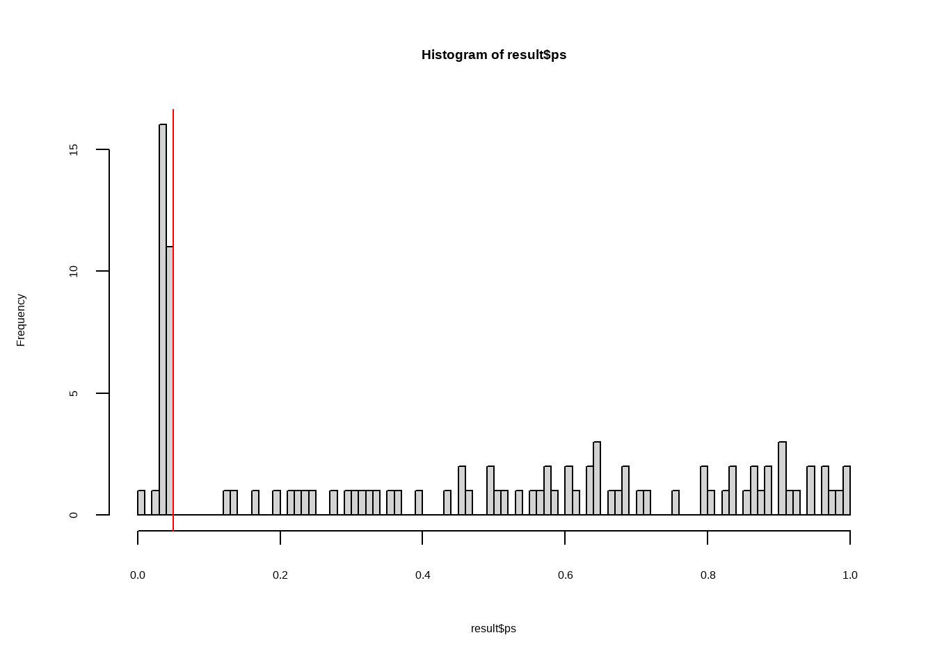
# Type 1 error rate
mean(result$ps <.05)
## [1] 0.29
Now type 1 error rate when final p-value is extracted.
# Obtain last p-value
result <- results_df %>%
  group_by(dataset) %>%
  summarize(ps = tail(ps, 1)) %>%
  ungroup()


# Create histogram
hist(result$ps, breaks = 100)
abline(v=.05,col="red")
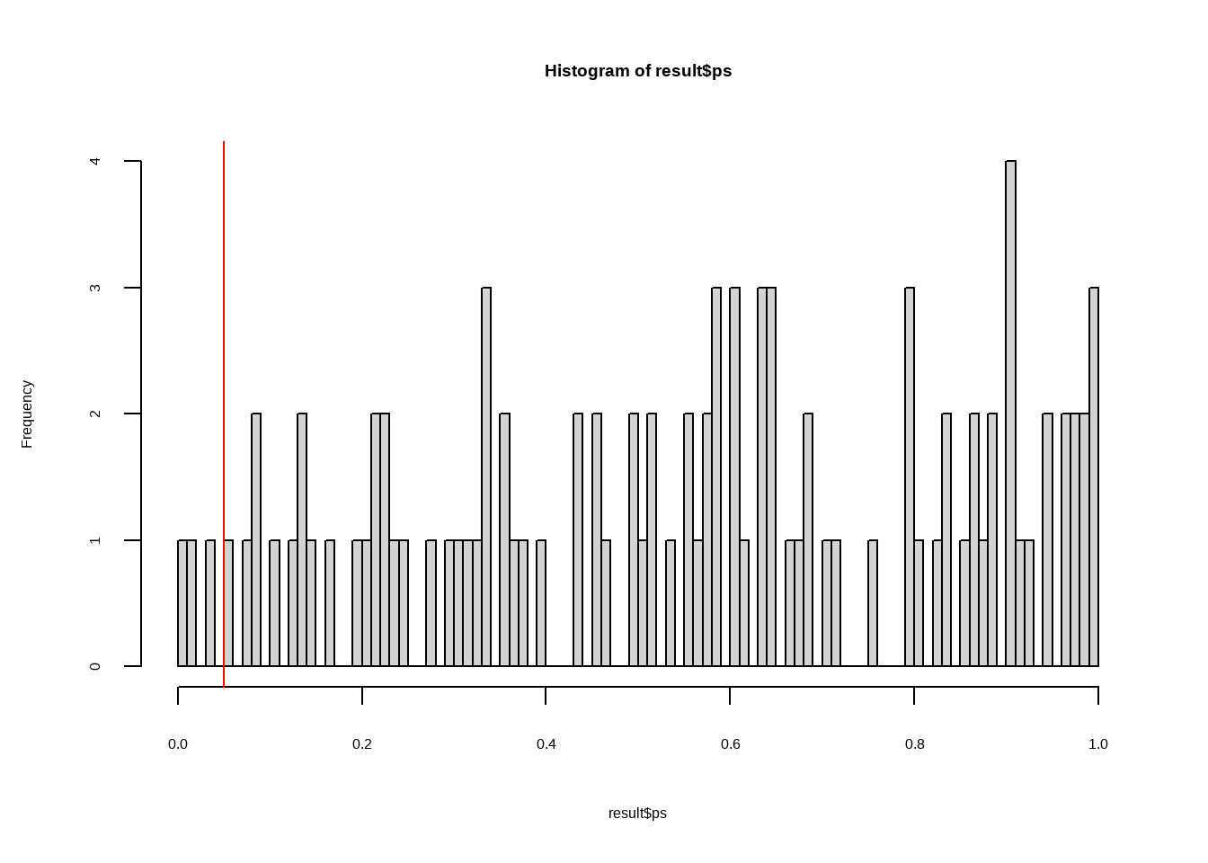
# Type 1 error rate
mean(result$ps < .05)
## [1] 0.03
Type 1 error rate - Safe testing
First check what the type 1 error rate is if researchers stop after the first e-value above 20 or the last e-value
# Filter each dataset to get either the first e-value above 20 or the last e-value
result <- results_df %>%
  group_by(dataset) %>%
  filter(evs == ifelse(any(evs > 20), head(evs[evs > 20],1), tail(evs, na.rm = TRUE,1))) %>%
  ungroup()

# Create histogram
hist(result$evs, breaks = 100)
abline(v=20,col="red")
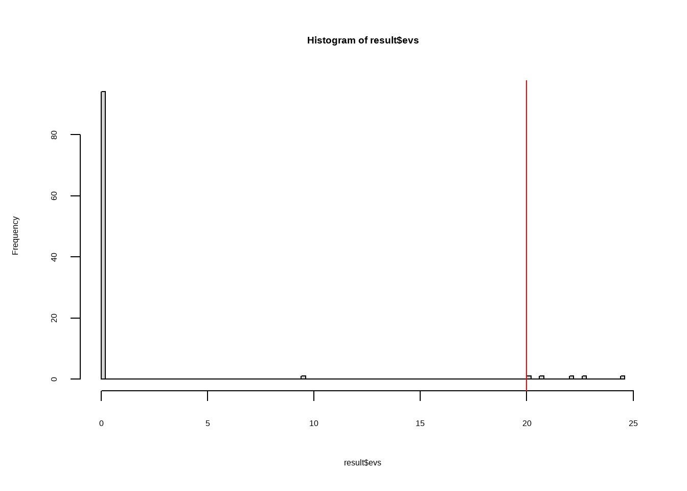
# Type 1 error rate
mean(result$evs > 20)
## [1] 0.05
Only take final evs-value
result <- results_df %>%
  group_by(dataset) %>%
  summarize(evs = tail(evs, 1)) %>%
  ungroup()

hist(result$evs, breaks = 100)
abline(v=20,col="red")
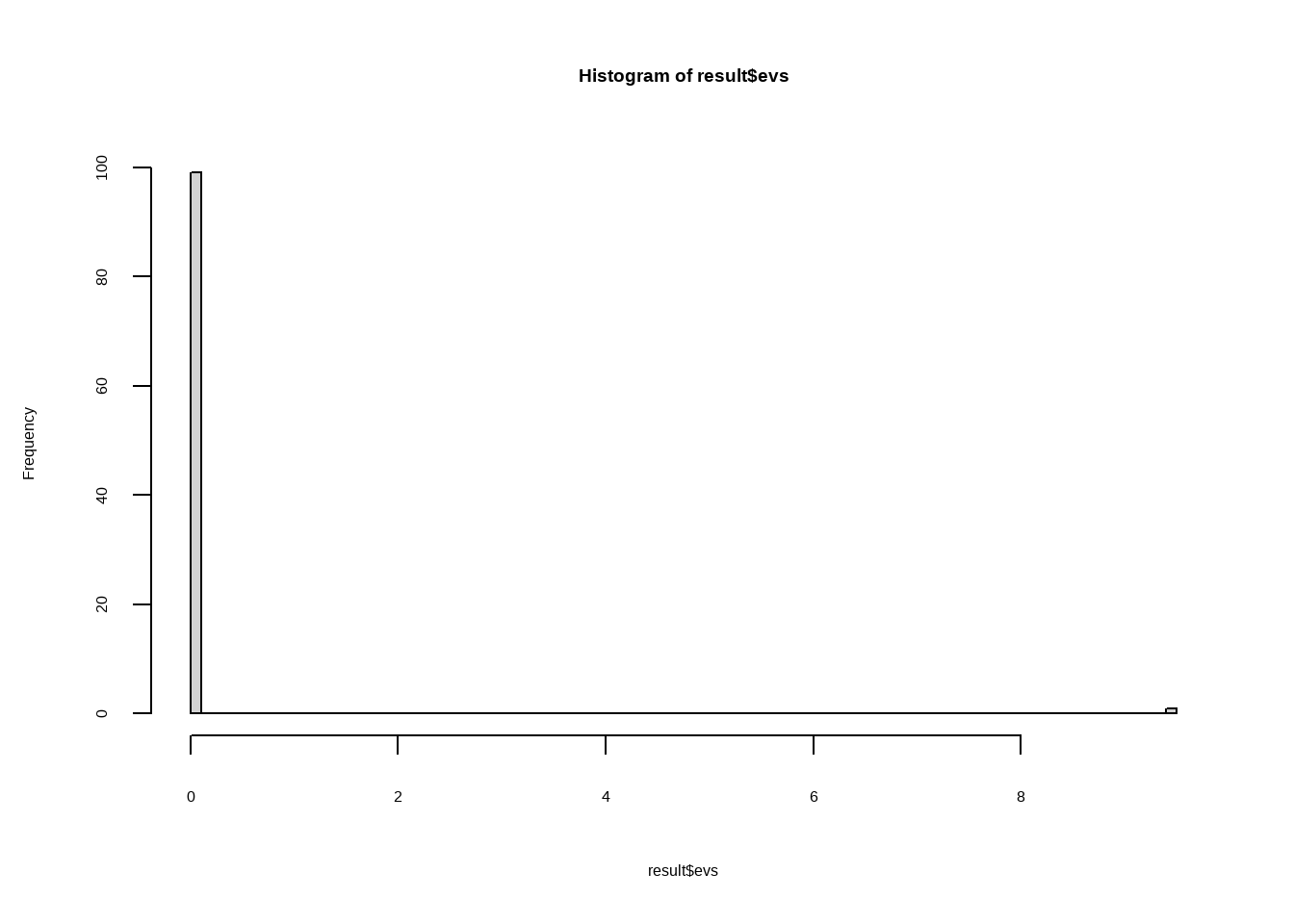
mean(result$evs > 20, na.rm=T)
## [1] 0
Plot estimates of each 95%CIs and CSs when first e-value is extracted
result <- results_df %>%
  group_by(dataset) %>%
  filter(evs == ifelse(any(evs > 20), head(evs[evs > 20],1), tail(evs, na.rm = TRUE,1))) %>%
  ungroup()

ggplot(result, aes(x = dataset))+
  geom_point(aes(y = L95, colour = "green"))+
  geom_line(aes(y = L95), col = "green")+
  geom_point(aes(y= H95, colour= "green"))+
  geom_line(aes(y = H95), col = "green")+
  geom_point(aes(y = L952, colour="red"))+
  geom_line(aes(y = L952), col = "red")+
  geom_point(aes(y= H952, colour="red"))+
  geom_line(aes(y = H952), col = "red")+
  geom_point(aes(y = est, colour="blue"))+
  geom_line(aes(y = est), col = "blue")+
  scale_colour_manual(values = c("blue", "green", "red"),
                      name = "Values",   # Change this to your desired legend title
                      labels = c("Estimate", "95%CS", "95CI")) + # Custom labels
  labs(title = "Estimates and 95% Confidence Intervals and Sequences",  # Change this to your desired plot title
       x = "Dataset",                     # Custom x-axis label
       y = "Raw mean differences") +                     # Custom y-axis label
  scale_x_continuous(breaks = seq(0,1000,50),expand = expansion(mult = c(0, 0.05))) +
  scale_y_continuous(breaks = seq(-2,7,.5)) +
  transition_reveal(seq_along(dataset)) + shadow_mark()+
  theme_barbie()
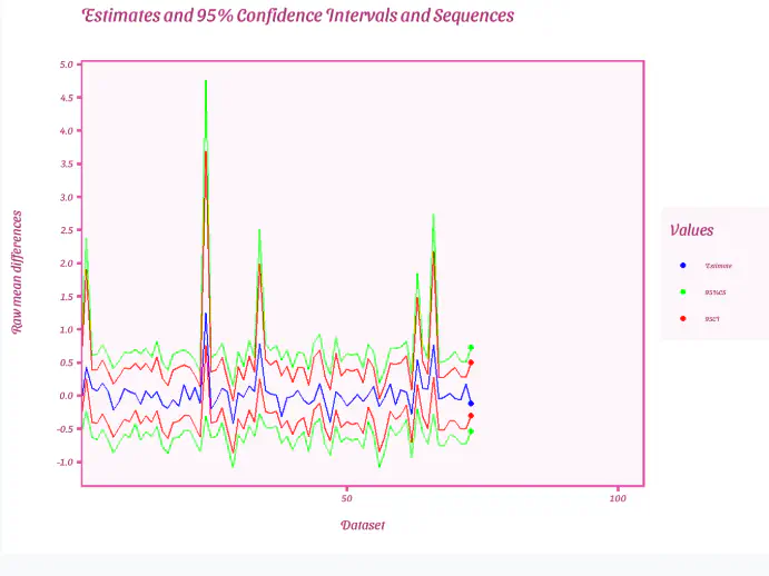
Plot estimates of each 95%CIs and CSs when last e-value is extracted
result <- results_df %>%
  group_by(dataset) %>%
  filter(evs == tail(evs,1)) %>%
  ungroup()

ggplot(result, aes(x = dataset))+
  geom_point(aes(y = L95, colour = "green"))+
  geom_line(aes(y = L95), col = "green")+
  geom_point(aes(y= H95, colour= "green"))+
  geom_line(aes(y = H95), col = "green")+
  geom_point(aes(y = L952, colour="red"))+
  geom_line(aes(y = L952), col = "red")+
  geom_point(aes(y= H952, colour="red"))+
  geom_line(aes(y = H952), col = "red")+
  geom_point(aes(y = est, colour="blue"))+
  geom_line(aes(y = est), col = "blue")+
  scale_colour_manual(values = c("blue", "green", "red"),
                      name = "Values",   # Change this to your desired legend title
                      labels = c("Estimate", "95%CS", "95CI")) + # Custom labels
  labs(title = "Estimates and 95% Confidence Intervals and Sequences",  # Change this to your desired plot title
       x = "Dataset",                     # Custom x-axis label
       y = "Raw mean differences") +                     # Custom y-axis label
  scale_x_continuous(breaks = seq(0,1000,50),expand = expansion(mult = c(0, 0.05))) +
  scale_y_continuous(breaks = seq(-2,7,.5)) +
  transition_reveal(seq_along(dataset)) + shadow_mark()+
  theme_barbie()
Calculate power for normal evalues, minimum-effect testing, and equivalence testing
result <- results_df %>%
  group_by(dataset) %>%
  filter(evs == tail(evs,1)) %>%
  ungroup()

power_normal <- data.frame(
  "NHST" = mean(result$ps < .05, na.rm=T),
  "ET" = mean(result$L952 > -SESOI & result$H952 < SESOI, na.rm=T),
  "ME" = mean(result$L952 > SESOI | result$H952 < - SESOI, na.rm=T))

power_normal
##   NHST   ET ME
## 1 0.03 0.47  0
power_safe <- data.frame(
  "NHST" = mean(result$evs > 20, na.rm=T),
  "ET" = mean(result$L95 > -SESOI & result$H95 < SESOI, na.rm=T),
  "ME" = mean(result$L95 > SESOI | result$H95 < - SESOI, na.rm=T))

power_safe
##   NHST ET ME
## 1    0  0  0